Skills and Scores

The ELO rating

For many years sanctioned tournament Magic used ELO rating as a tool to capture the skill level of each single player. Each players rating was thereby represented through a score which increased and decreased with every win and loss, respectively. ELO functions such that each players rating moves in the region around the player’s “true” rating, thus being a rough indicator of the players skill. Eventually, the DCI binned ELO since the rating was also used to hand out, e.g., PT qualifications which somewhat misused ELO as a bonification tool, which led to undesired side effects such as players not wanting to play in order to preserve a high rating. For those of you who didn’t get to know ELO from Magic, ELO also had its 15 minutes of fame during the opening scene in The Social Network: “I need the algorithm!”.

Figure 1: Scene from “The Social Network”

The mathematical principle of the rating system itself is rather straightforward. Given a match between players A and B with ratings \(x_A\) and \(x_B\), respectively, the ELO system models the win probability of player A as \[p_A = \frac{1}{1 + 10^{-(x_A - x_B) / c}},\] where \(c\) is some scaling constant (The DCI used \(c = 400\), I believe). From a statistical perspective, this corresponds to the predicted success probability from a logistic regression model using the rating difference (scaled through \(c\)) as its only covariable. Given the outcome of the match, player A’s rating increases by \(K \cdot(1-p_A)\) if he wins the match or decreases by \(K\cdot p_A\) if he loses, where \(K\) is some velocity factor. Thus, assuming the ELO predicted win probability is accurate, the expected rating change of player A is \[\mathbb{E} \left[\Delta x_A\right] = p_A \cdot K(1-p_A) + (1-p_A)\cdot(-Kp_A) = 0.\] Otherwise, if player A is underrated, i.e. its actual win probality is larger than \(p_A\), then the expected rating change is positive. If player A is overrated the expected rating change is negative. Thus, the rating tends to correct itself.

The relevant property for us is that ELO provides a predictive model for the outcome of any match between two players. All we need is the “true” ELO rating for both of these players. In fact, for our purposes we are interested in the distribution of the “true” ELO ratings within a GP player field, which will be addressed later.

MTGELOPROJECT data

To appy the ELO model, we need information on the actual ratings of the typical player field within a GP or PT. This is where the work of MTGELOPROJECT is crucial for us.

MTGELOPROJECT.net is a website created by Adam and Rebecca in order to reunite ELO and Magic: the Gathering. Based on published match results from each Grand Prix and Pro Tour since 2008 (or even earlier), the website retrospectively computes the ELO rating of each player appearing in the data. Scraping these data together sounds like an awful lot of work and it probably is. However, the result is a huge database with insightful statistics, where every player can check her current rating in progress. I highly recommend checking out the site, if you don’t know it yet.

Some time ago, I asked Adam whether he could provide some numbers on the typical rating distribution of a PT and GP player field. He sent me the following numbers (Thanks, Adam!):

• The mean player rating at a Grand Prix is 1554 with lower and upper quartiles of 1472 and 1606, respectively.

• The mean player rating at a Pro Tour is 1788 with lower and upper quartiles of 1660 and 1918, respectively.

To give a crude interpretation guideline: within MTGELOPROJECT each player starts at a rating of 1500. Thus, the GP player field is already above average. Also they use a scaling factor of \(c= 1136\), which means that a rating advantage of 200 points is equivalent to a win probability of 60%. Under the assumption of a normally distributed rating within each tournament player field, I used the interquartile range to roughly compute the corresponding standard deviations which led to the following rating distributions:

• At a Grand Prix the rating is normally distributed with mean 1554 and standard deviation 100.

• At a Pro Tour the rating is normally distributed with mean 1788 and standard deviation 200.

These are the eventual rating distribution which I applied within the ELO model. Before we come to that, two things should be remarked:

1. The mean rating within a PT is much higher compared to a GP, which is of course expected.

2. The standard deviation, i.e. the rating differences within the player field, are much higher in the PT compared to the GP. I guess this a consequence of many GP players not yet being rated to their true skill within the data, since an accurate rating takes many matches. In contrast, the typical Pro Tour player has already played a few dozens of matches on the GP and PT level, which is why I think that these ratings are roughly accurate. However, this is pure gut feeling and the GP player field might in fact be much more dense with respect to skill level.

Simulating player fields by score brackets

It’s time to go off. Using (i) the data on the player field rating distribution and (ii) the ELO model to estimate win probabilities based on those ratings we are now ready to simulate a virtual Grand Prix tournament. Based on this simulation we can draw conclusions on how the rating distribution varies by score bracket as the tournament goes on,

To simulate the tournament, I used the following algorithm which I implemented using R. Here, let \(N\) be the number of tournament players with individual ratings \(x_i\) (\(i=1,\ldots, N\)) drawn independently from a normal distribution with mean 1554 and standard deviation 100 (the GP rating distribution as given above). Let \(r^{(j)}_i\) (\(i=1,\ldots, N\)) denote the number of wins of player \(i\) after round \(j\). For the sake of definedness we set \(r^{(0)}_i = 0\) for all players. Then we apply the following algorithm:

1. For \(j = 1, \ldots, 9\) repeat the following steps 2) to 4).

2. Sort all players by descending \(r^{(j-1)}_i\) (i.e we sort by score). In case of ties sort randomly within the tie brackets.

3. Based on this sorting order, generate pairings by matching player 1 against player 2, player 3 against player 4, and so on. (This procedure basically produces swiss pairings. For simplicity we chose \(N\) to be an even number.)

4. For each of the \(N/2\) round matches do the following: let’s denote the two participating players by \(i_1\) and \(i_2\). We compute the win probability of player \(i_1\) by applying the ELO formula \(p = (1 + 10^{-(x_{i_1} - x_{i_2}) / c})^{-1}\) with \(c = 1136\). Draw \(Y \sim\) Bern\((p)\) from a Bernoulli distribution (basically we throw a coin that shows head (Y=1) with probability \(p\) and tails (Y=0) with probability \(1-p\)). In case of \(Y=1\) we set \(r^{(j+1)}_{i_1} = r^{(j)}_{i_1} + 1\) and \(r^{(j+1)}_{i_2} = r^{(j)}_{i_2}\) (i.e. player \(i_1\) receives a win). In case of \(Y=0\), update analogeously such that player \(i_2\) receives the win.

5. Discard all players with \(r^{(9)}_i < 6\). (We make a cut after nine rounds and continue only with players who received six wins)

6. Using the diminished player field repeat steps 2) to 4) for \(j = 9, \ldots, 14\).

Note that for this Grand Prix simulation we did not update the rating of each player after each round, since we are only interested in the rating as an indicator for each player’s fixed skill level and not in the rating fluctuations themselves. After the dust is settled, our simulated tournament results contain the number of players within each score bracket after each round and more importantly the ratings of these players within the individual brackets. These bracket specific rating distributions provide a clear picture on how your skill level can affect your tournament score. For instance, let’s look at a snap shot after round nine from a simulation with \(N = 10000000\) players.

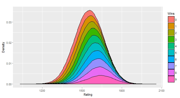
Figure 2: Rating distribution (given as stacked densities) after round nine of a GP stratified by score.

Here, we see the overall rating distribution of the whole player field and how the player field is decomposed into the different score brackets from zero to nine wins. One can see, that the mean rating of the players with six or more wins – thus reaching day 2 – is at around 1600 (much lower than the mean rating at PT level). The mean rating of the 9-0 players is at around 1650. From another perspective one can also see, that most players rated at 1650 reach day 2 by looking at the “vertical”, i.e. conditional, distribution along the 1650 rating line.

The win probability tree

So far we looked at a model to translate any rating into a win probability against any other opponent rating. Also, due to our simulated tournament based on empirical data we know the players rating distribution within each possible score bracket. By bringing these components together, we are now able to compute the expected win probability of any rated player within a certain score bracket of, e.g., a Grand Prix.

The notation will get a little technical now. To calculate the expected win probability we need to take a look at the simulated player ratings within a specific score bracket. Based on simulated results from above let’s denote by \[\mathcal{R}^{(j)}_w = \{x_i | r^{(j)}_i = w \}\] the rating sample of those players with exactly \(w\) wins after \(j\) rounds. We denote by \[\bar{r}_w^{(j)} = \text{mean}(\mathcal{R}^{(j)}_w), \quad \text{and} \quad \sigma_w^{(j)} = \text{Var}(\mathcal{R}^{(j)}_w)\] the emprical mean and variance of this rating sample. The expected win probability on a player with rating \(x\) within the score bracket “\(w\) wins after \(j\) rounds” can then be approximated by \[p_w^{(j)} (x) \approx \left|\mathcal{R}^{(j)}_w\right|^{(-1)} \sum_{y \in \mathcal{R}^{(j)}_w}\frac{1}{1 + 10^{-(x - y)/c}}\] \[\approx \int_{\mathbb{R}} \frac{1}{1 + 10^{-(x - y) / c}} \, \varphi(y, \bar{r}_w^{(j)}, \sigma_w^{(j)}) dy,\] where \(\varphi(\cdot, r, \sigma)\) denotes the density of a normal distribution with mean \(r\) and variance \(\sigma\). This integral is a rather complicated way to write the solution for the following calculations:

1. What are frequent ratings within in the score bracket “\(w\) wins after \(j\) rounds”?

2. What are the win probabilities against those ratings?

3. What is the resulting average win probability?

This formula gives a translation rating into win probability“. Conversely, for a given score bracket and a given win probability within this bracket we can compute the virtual rating that corresponds to that win probability. To do so, one has to find the rating \(x^*\) such that \[p_w^{(j)} (x^*) = p^*,\] where \(p^*\) is the desired win probability. This equation can be easily solved numerically (read: it cannot be solved easily).

Now it’s time to reap the rewards. By applying a certain rating to all possible score brackets within a GP we obtain all respective win probabilities. As the tournament progresses these score dependent changes in the expected win probability per round thus form a shape of a tree branch as seen below. For this example graphic I set the protagonist’s rating to 1554, i.e. the mean rating in a GP. The underlying rating parameters to produce this tree were those from the MTGELOPROJECT data given above.

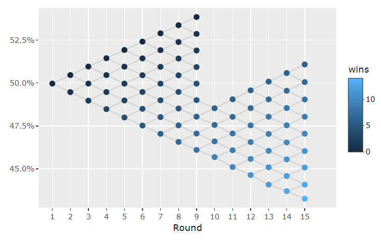
Figure 3: Win probability tree for an average GP player.

For each round and score – given trough the number of wins – the tree shows (on the Y-axis) the expected win probability of the protagonist for the following round. In the above graphic the round one win probability is at exactly 50%, since the protagonists rating equals the mean rating in the player field. However, in round six at a score of 5-0 the expected win probability of the protagonist would be 47.5% due to the more skilled opponents within this bracket.

Since it’s not convenient to show all win probability trees (WPTs) for a large sprectrum of protagonist ratings and tournament forms within this post, I wrote a web application using R shiny in order to compute the WPT for any desired parameters. This WPT app can be found here:

[https://mtganalyze.shinyapps.io/wp_tree/]

As a user one can choose the tournament structure (GP or PT), the overall win probability against the field, and the skill density. A normal skill density corresponds to that from the MTGELOPROJECT data, whereas the dense and diverse skill density assume a smaller and larger variance in the rating distribution, respectively. As said above, for GPs I can imagine that the diverse skill density is closer to the true distribution. The app then computes the virtual MTGELOPROJECT rating and the corresponding WPT. One approach might be to chose the win probability such that it matches your own WPT rating. Just give it a try.

End of turn

I hope you enjoyed this first post. Maybe even you found it useful. I am very eager to hear your feedback. Do you like the idea of the WPT or do you think its abstract nonsense? Was the presentation too technical, too lengthy, too boring? I am happy to adjust for further content.

Next time, I will present an use case of the WPT, that especially for tournament players might be interesting. If you don’t want to miss it, follow me on twitter or just come back regularly.