“What is the most important concept that Limited players should strive to understand?”.
Ben Stark: “Not being too fancy. Most games are won or lost by hitting your mana curve.”
In his Limited Information column Marshall Sutcliff once interviewed Ben Stark on limited advice. This particular piece was dubbed “THE TRUTH” and Ben Stark was spitting it. As one of his main messages Ben was pointing out the importance of having a mana curve. Although many experienced and succesful limited players would immediately agree that a smooth mana curve is a necessacity for a good draft or sealed deck, it is very difficult to precisely nail down what makes a good curve. There are some rules of thumb, but beyond that there is no clear criteria to compare two decks in order to say which one has a “better” curve. Thus, this post’s topic is:
What are possible quantitative measures to define a good mana curve?
It is not very surprising that Frank Karsten already took a stab at this problem by searching for optimal mana curves via computer simulation for various contstructed formats. (I promise, my next topic will be one that Frank has not already fully covered.) Frank Karsten’s approach is as always clever and convenient. He separated the problem into two parts: (1) how does a particular mana curve translate into an in-game curve and (2) how can we assess the value of any particular in-game curve? Here I like to pick up this approach and especially I want to add and discuss possibilities regarding the second part. Like in my last posts the untiring reader will get rewarded with a ready-to-use web application to evaluate the mana curve of any limited deck.
(This post is written with limited deck building in mind. However, all concepts can be easily applied to any contructed format.)
From mana curve to curving out
When building a draft or sealed deck the typical procedure is to lay out your cards according to converted mana costs: with one pile of all one-drops, one pile of two-drops, and so on, from left to right (or from right to left if you like to see the world burn). This approach provides a quick overview over the number of cards in each mana cost slot in order to identify bumps in this so-called mana curve. It is common knowledge that a smooth curve with a priority on two-, three- and four-dops is generally a good indicator for your deck’s ability to actually curve out, which is to actually play those spells in your second, third and fourth turn of the game, respectively. This exact relation between your mana curve and your executed curve within a game however is hard to grasp and will be subject of this section.
What you can frequently observe is players goldfishing with their newly built deck. They draw an opening hand from their shuffled library, play lands, draw cards and unopposedly deploy their spells. By doing so these players go to the next level and get a feel for the actual executed curve of their deck. This is still only a rough approximation of the in-game curve since your actual sample size is pretty low. However, this method does not require any actual play skills. So why shouldn’t your nearest computer or mobile phone do this for you?
Figure 1: Copyright owned by Wizards of the Coast
The following algorithm does exactly that. For a given decklist it calculates the mean executed curve, i.e. the average amount of mana your deck is capable to spent on spells on each specific turn. In order to not depend on strategic advice and to keep it simple, the algorithm works with some assumptions on your deck though:
You only play proactive, unconditional spells. If the computer dummy notices that you can pay the mana cost of a spell, it will cast that spell. Fortunately, this “strategy” is valid for most types of spells such as creatures, direct damage, or to a lesser extent for enchantments and removal.
All your spells have an immediate effect on the game. If you cast spells that don’t affect the board such as Divination or Rampant Growth it’s hard to argue that these spells directly contribute to your executed curve. Thus, we assume that every spell in your deck and therefore every mana you spent goes directly into board development. In CABS Theory there is even an acknowledged strategy that propagates this play style.
All your spells are colorless. This is admittedly a very crude assumption, especially for limited decks, but it makes calculating the executed curve so much easier.
Another important property of the algorithm is that it is contained in a newly created grey math box. As suggested by one of the readers, from now on I will try to present any formulas or overly technical paragraphs in such an environment, which hopefully will make my posts more readable for those who like to skip the mathy stuff.
Algorithm: Mean Executed Curve
Let \(x_i\) denote the number of cards with converted mana cost \(i, (i=1, \ldots,n)\) up to a maximum cost of \(n\). Let \(d\) denote your overall deck size, i.e. \(d = 40\) for serious draft decks. The number of lands \(l\) is thus given by \(l = d - \sum_{i=1}^n x_i\). Let \(\mathbf{s} = (s_1, \ldots, s_d)\) be a random permutation of your deck with \(s_i\) taking values in \(\{0,\ldots, n \}\), i.e. \(\mathbf{s}\) is a shuffled version of your dech where \(s_i\) denotes the converted mana cost of the \(i\)-th card in your shuffled deck and mana costs of zero refer to a land. Let \(\mathbf{s}\) be the input of the following algorithm using a predefined number of turns \(T\):
Let \(\mathcal{H}_0 = \{s_1, \ldots, s_7\}\) be the first seven cards of your deck, i.e. your starting hand. Apply mulligans if necessary\(^*\). Let \(l_t\) denote your number of lands on the battlefield after turn \(t\), with \(l_0 = 0\).
For \(t = 1, \ldots, T\) repeat steps 3) to 6).
Draw a card, i.e. put the top card of your library into your hand \[\mathcal{H}^{(d)}_{t} = \mathcal{H}_{t-1} \cup \{s_{7+t}\}\]
Play a land if possible: If there exists an \(s \in \mathcal{H}^{(d)}_{t}\) with \(s = 0\), then set \(l_t = l_{t-1} + 1\) and \[\mathcal{H}^{(l)}_{t} = \mathcal{H}^{(d)}_{t} \setminus \{s\}.\] Otherwise set \(\mathcal{H}^{(l)}_{t} = \mathcal{H}^{(d)}_{t}\) and \(l_t = l_{t-1}\).
Play spells from your hand: Let \(m = l_t\) be the available amount of mana in this turn \(t\). Let \(\bar{s}^{(1)}\) be the highest mana cost of all spells that are castable, i.e. \[\bar{s}^{(1)} = \max\{s | s \in \mathcal{H}^{(l)}_{t}, s \leq m\}.\] If \(\bar{s}^{(1)} < m\), then let \(\bar{s}^{(2)}\) be the highest combined mana cost of any two spells that are castable simultaneously in this turn, i.e. \[\bar{s}^{(2)} = \max\{s + r | s,r \in \mathcal{H}^{(l)}_{t}, s+r \leq m\}.\] If \(\bar{s}^{(1)} \geq \bar{s}^{(2)}\), then set \(y_t = \bar{s}^{(1)}\) to be the amount of mana you spent this turn and update your hand via \[\mathcal{H}^{(s)}_{t} = \mathcal{H}^{(l)}_{t} \setminus \{s\},\] where \(s\) is a spell with mana cost \(\bar{s}^{(1)}\). Otherwise, set \(y_t = \bar{s}^{(2)}\) and \[\mathcal{H}^{(s)}_{t} = \mathcal{H}^{(l)}_{t} \setminus \{s,r\},\] where \(s,r\) are spells from your hand with combined manacost \(\bar{s}^{(2)}\). Then, if \(m - y_t > 0\) repeat step 5) with available mana \(\tilde{m} = m - y_t\) and add the spent mana to \(y_t\). Repeat this procedure until can’t cast any more spells from your hand.
Set your end of turn hand, i.e. \[\mathcal{H}_{t} = \mathcal{H}^{(s)}_{t}\]
As output from this algorithm one obtains a sequence \(\mathbf{y} = (y_1, \ldots, y_T)\) which represents the amount of mana that is spent each turn given the permutation \(\mathbf{s}\). Since the permutation of the deck is actually a random quantity the corresponding sequence \(\mathbf{y}\) and its components \(y_t\) are also random variables. In order to get a Monte Carlo estimate for the expected mana spent \(\bar{y}_t = \mathbb{E}[y_t]\) in each turn, one applies the above algorithm to a large sample of deck permutations \(\mathbf{s}^{(i)}, (i=1,\ldots,N)\) with corresponding results \(\mathbf{y}^{(i)}\). Then the mean executed curve is computed componentwise by \[ \bar{y}_t = N^{-1} \sum_{i=1}^{N} y_t^{(i)}.\]
\(^*\)The mulligan strategy is to mulligan any seven or six card hand with fewer than two lands or fewer than two spells. Any five card hand will be kept. Mulliganing means that the algorithm is started over with a new deck permutation and one fewer card in hand.
This algorithm performs pure goldfishing, playing spells from the hand as early as possible and counting how much mana is spent each turn doing so. Iterating this many thousand times gives a good grasp on how much mana a deck is capable to spent on average in each specific turn.
The algorithm is very similar to that of Frank Karsten. I only skimmed over his code, so please correct me if I’m wrong, but i believe there are two meaningful (but not huge) differences. Firstly, the procedure to select which spells to cast is much simpler in Frank Karsten’s version, in which only the one most expensive spell among all castable spells is cast each turn whereas the above algorithm checks additionally if there are any better two-card combinations and also looks if remaining mana can be spent on some cheaper spells in the hand. Secondly Frank Karsten uses a much more sophisticated mulligan rule derived through Stochastic Programming. My mulligan rule applied here is pure heuristic.
Let’s take a look at how the algorithms performs by applying it to an example deck, which i call the Wall of Mana. The Wall of Mana consists of four cards of each converted mana cost from one to six and sixteen lands. This decks mana curve is graphically presented below (upper figure).
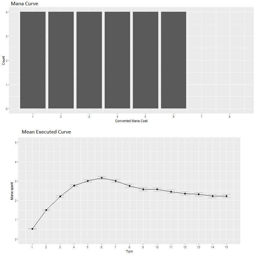
Figure 2: Mana curve and mean executed curve of the “wall of mana”
The lower figure provides the corresponding mean executed curve as computed by the algorithm above. For each turn the respective average mana spent is plotted together with confidence intervals regarding the estimate for the mean. This deck reaches its peak in turn six with on average 3.2 mana spent. For turns seven and higher the expected spent mana decreases to around 2.2, which represents the average mana costs of the top card of the library, since the deck is likely in top deck mode by then.
Evaluate the Curve
Although computing the mean executed curve requires some computer power, this is actually the somewhat easy task, because there exists a clear solution to the problem. Within this section we will deal with the problem on how to evaluate a given executed curve, which will not be as straightforward.
The main difficulty of this problem is to condense the mean executed curve consisting of mulitple variables – i.e. the expected amounts of mana spent in turns one, two, and so on – to one single number measuring the “power” of the curve. Thus, decks with good executed curves should obtain higher scores, whatever “good” means in this context?! Frank Karsten approached this problem by calculating the total amount of mana spent in the first X turns, where X was some value between three and six. His argument was, that in any specific constructed format from Modern to Block Constructed there exists a critical turn in which (on average) the game is actually or virutally over in the sense that it is clear which player is going to win the game. For instance, in Modern the winner should be determined after on average four turns, for Standard this would take five turns.
Although I think this method is a little too simple, the overall approach of calculating an index is very reasonable. An index is a function which summarizes multiple measures into one single score. For instance, Frank Karsten constructed his index (the K-index from now on) as the sum of mana spent in the first X turns whereas mana spent in every further turn is not accouted for. Moreover, although being very simple the K-index suggests two heuristics that any reasonable index function for mana curves evaluation should fulfill:
The more mana the better: The overall index score should not decrease, if the amount of expected mana increases for any given turn. Playing a Hill Giant should never be worse than playing Grizzly Bears.
The earlier the better: The overall index function should not decrease, if the same amount of spent mana is shifted to an earlier turn. Playing Grizzly Bears on turn two should be at least as good as on turn four. This heuristic acually accounts for two aspects. Firstly, especially for board affecting spells like creatures it’s always better to play them as early as possible in order to increase their impact on the game. Secondly, each game only lasts so many turns, which means that if your deck is capable of spending on average X mana on turn 10 it’s not guaranteed that you actually reach this turn in a given game. This decreasing probability to reach the later turns of the game should be accounted for.
In the following I want to present potential index functions to evaluated any given executed curve. For this purpose an index will be characterized through weights \(w_t\) which represent the relative impact of mana spent in each turn \(t\). Thus, if for instance an index has the weights \(w_1 = 1\) and \(w_2 = 0.8\), this means that this index will fully account for mana spent on turn one whereas mana spent on turn two has a shrinked impact with a factor of 0.8.
Index for Curve Evaluation
Let \(\mathcal{I}\) be an index function with weights \(\{w_t\}_{t=1,\ldots,T}\) up to turn \(T\). For any mean executed curve \(\mathbf{\bar{y}} = (\bar{y}_1, \ldots, \bar{y}_T)\) the index \(\mathcal{I}\) evaluates this curve through the weighted sum of spent mana, i.e. by \[\mathcal{I}(\mathbf{\bar{y}}) = \sum_{t=1}^T w_t\cdot \bar{y}_t.\] Translating the above mentioned heurstics into restrictions on \(\{w_t\}_{t=1,\ldots,T}\) in order to have a reasonable index \(\mathcal{I}\), we obtain the conditions \(w_t \geq 0\) for all \(t \in \{1,\ldots,T\}\) and \(w_t \geq w_s\) for \(t < s\).
(Note, that this is not the only possibility to construct suitable index functions, e.g. a more general approach would be to define \[\mathcal{I}(\mathbf{\bar{y}}) = \sum_{t=1}^T w_t(\bar{y}_t),\] for a family of functions \(\{w_t\}\) fulfilling the same restrictions, i.e monotony with respect to \(t\) and \(y\).)
So let’s look at some potential candidates for index functions and their associated weights.
K-Index
As introduced by Frank Karsten, the K-Index fully accounts for and sums up the mana spent within the first X turns and does not acount for any mana spent in subsequent turns. Thus, if for instance we set X=5 the respective weights would be \(w_1 = \ldots = w_5 = 1\) and \(w_6 = w_7 = \ldots = 0\). The corresponding weight curve is given below.
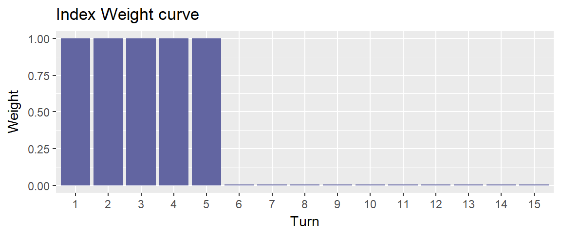
Although the K-Index provides a very simple first approach to evaluate executed curves, it has some weaknesses in my opinion. First of all, setting a specific critical turn at which the game is deemed to be virtually over is rather crude. While it might be correct that on average a game of Standard lasts five turns, that does not imply that every game of standard is finished after exactly five turns. However, according to the K-Index (X=5) everything you do after turn five is meaningless to the game, which I think is oversimplified. On the other hand, the first five turns are treated equally in the sense that there is no form of downgrading for mana spent in later turns. For instance, in current Standard a Bomat Courier is much more impactful on turn one in contrast to turn four or five. The K-Index does not account for that.
Full-Utilization-Index
The Full-Utilization-Index (FU-Index) picks up the idea that a good curve uses all available mana in every turn. A two-drop on turn two is of equal value as a four-drop on turn four. Thus, each turn is evaluated by measuring how much mana was spent in relation to the amount of mana that is potentially available in that turn. For instance, for turn two we are interested in the share of mana spent among the two available mana. This leads to the weights \(w_1 = 1\), \(w_2 = 1/2\), \(w_3 = 1/3\), and so on. These weights seem to put a high priority on the earlier turns, especially the first turn since each one mana in a given turn is only worth it’s share of the potentially available mana in that turn. See below for the corresponding weight curve.
At first glance, the FU-Index weight curve appears to be a reasonable weighting, where the correct strategy is likely to play many cheap spells in order to utilize the relatively impactful first few turns. However, this weight curve has the problem that in the later turns there is not enough further downgrading, e.g. a five drop has a high value on turn five but still also on turn six, seven or eight, whereas one-drops and two-drops have hugely diminishing impact. Moreover, since these weights are relatively stable after turn eight or nine, this does not reflect that it’s increasingly unlikely to actually reach any later turns. Thus, the actually correct strategy according to the FU-Index is to play a lot of high drops with a low land count in order to maximize the somewhat overvalued late game.
Discount-Index
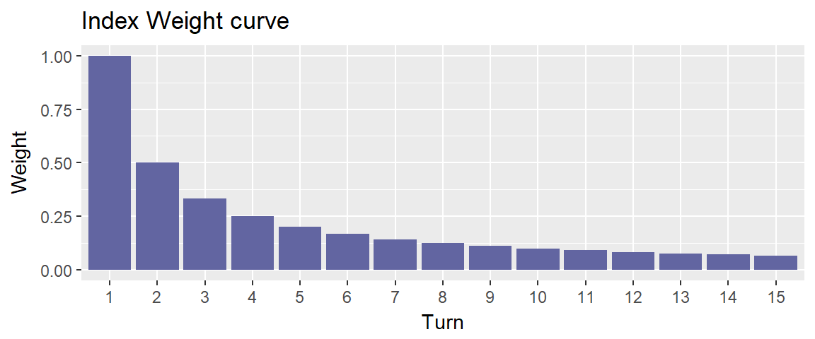
In economics one often uses discounting as a tool to adjust for the temporal delay of future incomes and outcomes. When discounting, the value of future payoffs is decreased by a certain discount factor for each time unit the payoff is delayed. Applying this concept to curve evaluation means that the value of one mana spent decreases each turn by the same factor \(d<1\), since the payoff you get from the mana is delayed correspondingly. This suggests the Discount-Index (D-Index) with weights \(w_1 = 1\), \(w_2 = d\), \(w_3 = d^2\), and so on. For a discount factor of \(d = 0.8\) the respective weight curve is given below.
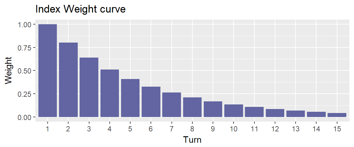
Figure 3: Weight curve of the D-Index using a discount factor of 0.8.
The D-Index weight curve looks very similar to that of the FU-Index, but there are some significant differences. First of all, the highest impact value of one mana is also given within the first turn. However, the relative loss of impact with each turn is constant over all turns, meaning that the relative difference between turns one and two is the same as between turns eight and nine. In contrast, the FU-Index suggested a rather big loss of impact within the first few turn, but a low impact decrease in the later turns. Thus, the D-Index actually somewhat captures both dynamics: i.e. (1) the decreasing impact of spells with each passed turn in the early game, but also (2) a constant chance that the game ends for any given turn in the late game, which motivates the steady relative decrease of the later turn weights.
Moreover, the D-Index is well scalable through its discount factor \(d\). A higher discount factor reflects slow discounting, which represents a small loss of mana impact over the turns combined with on average longer games. On the other and, low discount factors stand for short games with a large relative decrease of mana impact with each turn. Thus, by scaling the discount factor of the D-Index, one can easily control for which environment or format a given executed curve should be evaluated, since different indices actually imply different priorities in assessing the value of an executed curves. Overall, this makes the D-Index very suitable for curve evaluation.
The Curve Evaluator
Let’s do a quick recap. We looked at an algorithm, that for any given decklist in terms of a mana curve can calculate this deck’s average executed curve. Additionally, we looked at different ways in the form of index functions to evaluate such a mean executed curve. Unfortunately, the actual computation of especially the first part is rather tedious. I don’t want anyone to waste so much pencil and paper and since you probably have to do laundry anyway I’d like to present the Curve Evaluator that does all this work for you (the computations, not the laundry):
[https://mtganalyze.shinyapps.io/curveevaluator/]
The Curve Evaluator takes any 40 card limited deck with a mana curve up to a maximum mana cost of eight and calculates 1) the respective mean executed curve and 2) evaluates this according to the Discount-Index presented above. As there is not a single best D-index the Curve Evaluator applies the D-Index using six different discount factors: 0.55, 0.6, 0.65, 0.7, 0.75, and 0.8. This provides a range for assessing curves within the fastest of the fast limited formats (looking at you, Zendikar) or within the slow and grindy ones (Chaos Draft Hype!!!). Taking the Wall of Mana example from above, this is the resulting curve evaluation:
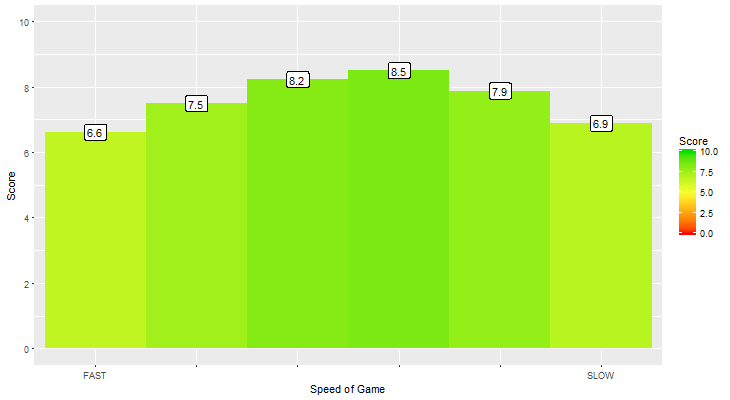
Figure 4: Curve evaluation scores of the “wall of mana”
As you can see, the curve evaluation does not provide the raw numbers from the different Discount-indices. Instead these results are transformed onto a zero-to-ten scale to be better interpretable, since the raw numbers don’t say much without further knowledge on the potentially optimal index results. To derive these easy to grasp and fancy looking zero-to-ten scales I computed for each underlying Discount-Index the best possible deck that produces an optimal result. (This will be the topic of my next post. SPOILER ALERT: there will be optimal mana curves!) Then, for any mana curve I put the corresponding index result in relation to the optimal result in order to compute a score between zero and ten. Thus, only the deck(s) which maximize a certain D-index reach a ten on the respective score.
Mana Curve Evaluation Scores
Let \(\mathbf{x}=(x_1, \ldots, x_n)\) be a decklist, where again \(x_i\) denotes the number of cards with converted mana cost \(i\), and let \(\mathbf{\bar{y}}(\mathbf{x})\) be the deck’s mean executed curve. Thus, for any index function \(\mathcal{I}\) we can define the index of \(\mathcal{I}(\mathbf{x})\) as the index of the deck’s mean executed curve \(\mathcal{I}(\mathbf{\bar{y}}(\mathbf{x}))\). Let \(\mathbf{x}^*\) be the decklist that maximises the index \(\mathcal{I}\) over all possible decklists. Thus, the best optimal index value is given by \(\mathcal{I}(\mathbf{x}^*)\).
Let \(\mathcal{S}\) denote the zero-to-ten score associated with the index \(\mathcal{I}\). For any decklist \(\mathbf{x}\) this score is computed by \[ \mathcal{S}(\mathbf{x}) = 10 \cdot \left( \frac{\mathcal{I}(\mathbf{x})}{\mathcal{I}(\mathbf{x}^*)} \right)^c,\] i.e. as ten times the fraction of the index of deck \(\mathbf{x}\) divided by the best possible index result. I also applied an additional power operation within the score function \(\mathcal{S}\), since I found a simple linear score didn’t provide enough penalization. For instance, a deck that spents only 70% as much mana as the optimal deck would still reach a score of 7.0, which to me is a rather good score given the actually bad performance of the deck. Thus, by introducing the power parameter \(c > 1\), the score is better able to penalize differences from the optimal value. For the purposes of the app I chose \(c = \pi\), because it looks very scientific.
One way to utilize the curve evaluator within a booster draft is to build a deck that aims to maximize one of the given scores. Which score to target is a question of the speed of the environment and the overall strategy of your deck. The more aggressive the format and your strategy, the more you should look at the “FAST”-Scores, i.e. the left bars of the chart. Personally, I have so far no practical experiences with the curve evaluator, but I am curious to find out whether it can provide tiebreaker insight for single card decisions.
End of turn
My main goal for this post was to provide tools to analyze a given mana curve, using computer simulation and index summaries. Especially the choice of a suitable index measure for eventual curve evaluation is highly subjective, and I am interested in what you think is a proper weighting of the individual turns in a limited game. On this regard but also with other goals in mind, there are many possibilities to build up on the here presented tools, e.g.:
With data on the game length distribution of a specific limited format, it could be possible to derive an index that directly accounts for the probability to reach any given turn. This would enable something like the “expected amount of mana spent per game”-Index.
Accouting also for mana color would enhance the deck evaluation, e.g. by assessing single card inclusions not only with respect to mana cost but also color requirements. Moreover, it would allow to determine the optimal land distribution for any given deck.
The impact of indirect effects such as a Divination is not yet covered by the executed curve simulator. By adding such a component one could analyze in which cases it is worthwhile to include such an effect in a deck and what are the consequences for building the remaining deck. For instance, do you actually play fewer or more lands in a deck with four Divinations?
If you have any further ideas or other comments on this topic, please let me no. Until then, my next post will deal with optimal decks regarding the here presented evaluation measures and how to find these decks.